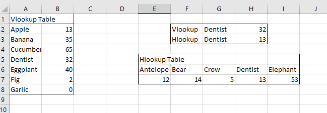
Two of the more useful functions in Excel and Google Sheets are the vlookup and the hlookup functions. Use these functions for finding values in a table that correspond to a specific value you’re looking for. You use vlookup for data stored in columns. You use hlookup for data stored in rows.

VLookup
For VLookup, you need 3 parameters. First, what is the lookup value? This is the value that you’re about to search the table for. Using the above example, I looked up G1, which at the time was just “Vlookup”. Then, you need to specify what array you’re looking in. One big caveat here is that your array needs to be continuous and the lookup value has to be the left most column. Finally, you need to pick the column number to return the value from.
In our above example, we would get an error because “Vlookup” isn’t one of the items in the table. You can protect your data against these kinds of errors by using the iferror function.

HLookup
For HLookup, you again need 3 parameters. The parameters are the same as before. However, they’re in rows instead of columns. Check out our above example. Using HLookup, I looked for “Dentist” in the below table. In this case, it returns 13.

Example
Recently, I ran an analysis of some of my blogs on another site. I used a vlookup function to pull data from an imported table from Google Analytics. Using that function, I was able to pull the pageviews for different blogs from tables. It doesn’t matter how those other tables are sorted. The lookup functions can pull from anywhere in a list.
Duplicates
Be very careful if your data has multiples. For example, if there are multiple “Dentist” entries in the list, I can’t tell you how the function picks which one to choose. Unfortunately, you only get one. If you want the sum of all the Dentists, you have to use a sumif.
How do you foresee yourself using these functions in the future?


Leave a Reply